This chapter assembles the pipeline step by step without YAML. It is the most explicit of the tutorials and is useful when you need custom logic that does not fit cleanly into a config file.
| Step | Input | Output |
|---|---|---|
| Search | (collections, intersects, start_datetime, end_datetime, **kwargs) | GeoDataFrame[AssetSchema] |
| Build | (GeoDataFrame[AssetSchema], ExtractionJob, **kwargs) | Sequence[ExtractionTask] |
| Read | (task: ExtractionTask, **kwargs) | xr.Dataset |
| Write | (ds: xr.Dataset, path: str, **kwargs) | str |
Use this chapter when you want to understand the mechanics underneath ExtractionJob, or when you need a custom pipeline that is hard to express in YAML.
Environment setup
The first cell installs AerEO and any required plugins. If you are reading the rendered book or running on Binder, where the environment is already prepared, pip will report that the requirements are satisfied and skip the download.
# Install AerEO and any required plugins for this notebook (Google Colab)
!pip install -q "aereo[viz]"
Imports and job construction
We import the low-level builtins directly: search_stac for discovery, build_grouped_tasks for splitting work, read_odc_stac for loading data, and write_geotiff for serialization. We also use shapely to define the AOI geometry inline, so this notebook has no external file dependencies.
The next cell builds an ExtractionJob in Python. This is equivalent to loading a YAML config, but every choice is explicit.
from aereo.builtins.search import search_stac
from datetime import datetime, timezone
from shapely.geometry import Polygon

from aereo.pipeline import ExtractionJob
from aereo.builtins import read_odc_stac, write_geotiff

# AOI polygon — Chocón reservoir, Argentina (inlined so the notebook has no file dependencies).
aoi_polygon = Polygon(
    [
        (-68.90986824592407, -39.23705421799603),
        (-68.65925870907353, -39.23705421799603),
        (-68.65925870907353, -39.41589522092947),
        (-68.90986824592407, -39.41589522092947),
        (-68.90986824592407, -39.23705421799603),
    ]
)

grid_dist = 10_000

job = ExtractionJob(
    name="sentinel2_sample",
    grid_dist=grid_dist,
    output_uri="/tmp/aereo_extraction",
    read=read_odc_stac,
    write=write_geotiff,
    target_aoi=aoi_polygon,
)
Step 1 — Search: search_stac
The search provider queries the STAC API and returns a GeoDataFrame of matched assets. Each row corresponds to one requested asset (e.g. red, nir) from one STAC item. All parameters are passed explicitly.
assets = search_stac(
    stac_api_url="https://earth-search.aws.element84.com/v1",
    collections={"sentinel-2-l2a": ["red", "nir"]},
    intersects=aoi_polygon,
    start_datetime=datetime(2024, 1, 1, tzinfo=timezone.utc),
    end_datetime=datetime(2024, 1, 10, tzinfo=timezone.utc),
)

print(f"\u2713 Found {len(assets)} asset rows")
print("Columns:", list(assets.columns))
print("First rows:")
assets[["id", "collection", "channel_id", "crs", "href"]].head()
✓ Found 12 asset rows
Columns: ['id', 'collection', 'geometry', 'start_time', 'end_time', 'href', 'channel_id', 'crs', 'stac_item']
First rows:
Step 2 — Build tasks: build_grouped_tasks
The task builder takes the search-result GeoDataFrame and the ExtractionJob and produces a list of ExtractionTask objects. Tasks are grouped by start time and native CRS, and chunked by cells_per_task.
from aereo.builtins.task_builder import build_grouped_tasks

tasks = build_grouped_tasks(
    search_results=assets,
    job=job,
)
print(f"\u2713 Built {len(tasks)} extraction task(s)")
for i, task in enumerate(tasks):
    print(f"Task {i}: {task}")
✓ Built 6 extraction task(s)
Task 0: ExtractionTask(id='sentinel2_sample_2024-01-02 14:33:47.691000_EPSG:32719_0', n_assets=2, n_grid_cells=10, read=True, write=True, output_uri='/tmp/aereo_extraction')
Task 1: ExtractionTask(id='sentinel2_sample_2024-01-02 14:33:51.276000_EPSG:32719_1', n_assets=2, n_grid_cells=4, read=True, write=True, output_uri='/tmp/aereo_extraction')
Task 2: ExtractionTask(id='sentinel2_sample_2024-01-05 14:43:42.172000_EPSG:32719_2', n_assets=2, n_grid_cells=10, read=True, write=True, output_uri='/tmp/aereo_extraction')
Task 3: ExtractionTask(id='sentinel2_sample_2024-01-05 14:43:46.672000_EPSG:32719_3', n_assets=2, n_grid_cells=4, read=True, write=True, output_uri='/tmp/aereo_extraction')
Task 4: ExtractionTask(id='sentinel2_sample_2024-01-07 14:33:42.975000_EPSG:32719_4', n_assets=2, n_grid_cells=10, read=True, write=True, output_uri='/tmp/aereo_extraction')
Task 5: ExtractionTask(id='sentinel2_sample_2024-01-07 14:33:46.552000_EPSG:32719_5', n_assets=2, n_grid_cells=4, read=True, write=True, output_uri='/tmp/aereo_extraction')
Inspecting a task
A task is a lightweight object that knows which grid cells to process, which assets to read, and which pipeline functions to apply. Printing it is a good way to verify that the search and grid parameters line up.
# Inspect the first task in detail
task = tasks[0]

print("Grid cells:", task.grid_cells)
print("Task context:", dict(task.task_context))
print(f"Number of asset rows in task: {len(task.assets)}")

# Extraction stages available on the task (delegated from the job)
print("Extraction stages:")
print("  read callable:", callable(task.job.read))
print("  write callable:", callable(task.job.write))
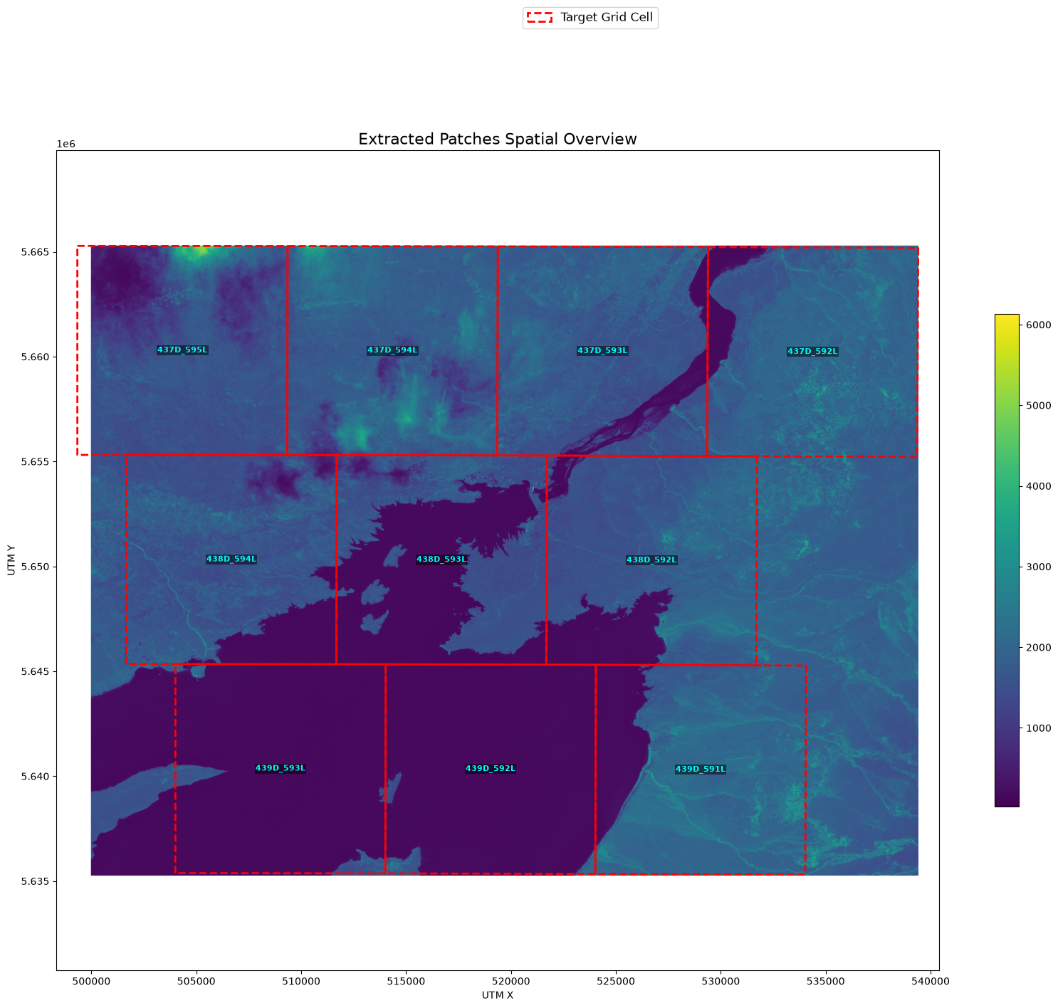
Grid cells: [GridCell(id='439D_593L', d=10000, cell_geometry=<POLYGON ((-68.837 -39.431, -68.837 -39.341, -68.953 -39.341, -68.953 -39.43...>), GridCell(id='439D_592L', d=10000, cell_geometry=<POLYGON ((-68.721 -39.431, -68.721 -39.341, -68.837 -39.341, -68.837 -39.43...>), GridCell(id='439D_591L', d=10000, cell_geometry=<POLYGON ((-68.605 -39.431, -68.605 -39.341, -68.721 -39.341, -68.721 -39.43...>), GridCell(id='438D_594L', d=10000, cell_geometry=<POLYGON ((-68.865 -39.341, -68.865 -39.251, -68.981 -39.251, -68.981 -39.34...>), GridCell(id='438D_593L', d=10000, cell_geometry=<POLYGON ((-68.748 -39.341, -68.748 -39.251, -68.865 -39.251, -68.865 -39.34...>), GridCell(id='438D_592L', d=10000, cell_geometry=<POLYGON ((-68.632 -39.341, -68.632 -39.251, -68.748 -39.251, -68.748 -39.34...>), GridCell(id='437D_595L', d=10000, cell_geometry=<POLYGON ((-68.892 -39.251, -68.892 -39.162, -69.008 -39.162, -69.008 -39.25...>), GridCell(id='437D_594L', d=10000, cell_geometry=<POLYGON ((-68.776 -39.251, -68.776 -39.162, -68.892 -39.162, -68.892 -39.25...>), GridCell(id='437D_593L', d=10000, cell_geometry=<POLYGON ((-68.66 -39.251, -68.66 -39.162, -68.776 -39.162, -68.776 -39.251,...>), GridCell(id='437D_592L', d=10000, cell_geometry=<POLYGON ((-68.544 -39.251, -68.544 -39.162, -68.66 -39.162, -68.66 -39.251,...>)]
Task context: {'chunk_index': 0}
Number of asset rows in task: 2
Extraction stages:
read callable: True
write callable: True
Step 3 — Read: read_odc_stac
The reader reconstructs pystac.Item objects from the asset table and uses odc.stac.load to build a lazy xarray.Dataset in the native CRS of the STAC items.
ds_native = job.read(task)

print("Native dataset:")
ds_native
# ds_native["red"].plot()
Native dataset:
Step 4 — Write: write_geotiff
The writer serialises a dataset to a GeoTIFF at the path supplied by the caller and returns the written path.
from pathlib import Path

# Write the native dataset to a temporary path
out_path = Path(job.output_uri) / "demo_native_red.tif"
# crate the parent directory if it doesn't exist
out_path.parent.mkdir(parents=True, exist_ok=True)
written = job.write(ds=ds_native, path=out_path)

print(f"\u2713 Wrote {written}")
✓ Wrote /tmp/aereo_extraction/demo_native_red.tif
Batch execution with an executor
For a single task the direct read/write API is fine. For many tasks, pass the task list to an Executor. The executor calls the read and write callables for each task, handles scheduling, and can run tasks in parallel.
Because this example reads cloud-optimized GeoTIFFs, LocalExecutor(use_threads=True) is a safe choice inside Jupyter and avoids the pickling issues that can make process pools hang.
from aereo.executors import LocalExecutor

# set job with partial functions for read and write
from functools import partial

# create a write partial function passing rioxarray/to_raster kwargs
write_partial = partial(write_geotiff, compress="LZW", tags={"creator": "aereo"})

job = ExtractionJob(
    name="sentinel2_sample",
    grid_dist=grid_dist,
    output_uri="/tmp/aereo_extraction",
    read=read_odc_stac,
    write=write_partial,
    target_aoi=aoi_polygon,
)

# lets build again the tasks with the new job
tasks = build_grouped_tasks(
    search_results=assets,
    job=job,
)

executor = LocalExecutor(workers=4, use_threads=True)
artifacts = executor(tasks)

print(f"\u2713 Extracted {len(artifacts)} artifact row(s) from {len(tasks)} task(s)")
artifacts[["id", "uri", "grid_cell", "start_time"]].head()
✓ Extracted 42 artifact row(s) from 6 task(s)
Verify the output
We reopen the first output GeoTIFF with rioxarray to confirm it has the expected bands, dimensions, and CRS.
# lets check that chunks are ok
import rioxarray

rioxarray.open_rasterio(artifacts["uri"].iloc[0])Visualize
Finally, plot_artifact_patches gives a quick map view of the extracted patches and the AOI.
from aereo.viz import plot_artifact_patches

plot_artifact_patches(artifacts, ds_factor=1, cmap="viridis")
(<Figure size 2000x1495.93 with 2 Axes>,
<Axes: title={'center': 'Extracted Patches Spatial Overview'}, xlabel='UTM X', ylabel='UTM Y'>)Ignoring fixed y limits to fulfill fixed data aspect with adjustable data limits.